Introduction
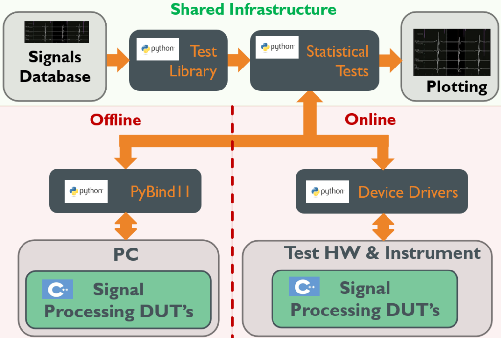
An integrated design and test (IDT) strategy involves executing design and development in a way that allows substantial reuse of engineering test development and verification infrastructure for both (a) offline design testing on a development platform, and (b) online physical testing often on an embedded system. Real-time signal processing building blocks inherently support this approach as illustrated in Fig. 1.

Figure 1: Integrated Design and Test Framework
The signal processing “devices” (C++ software) under test (DUTs) operate both offline on a PC and online in the target instrument hardware. If the shared test infrastructure is designed for real-time use, it can generate both simulated offline signals and physical signals—either through test hardware or direct communication with the instrument. Note that these tests are not only software unit tests but typically far more substantial statistical tests that may run for many hours processing databases of signals that provide important performance characterization.
This approach significantly reduces time and cost, as the design and development of complex statistical tests for offline characterization overlaps substantially with the engineering required for online implementation testing using physical hardware. By integrating C++ signal processing or algorithm test and verification for both design and hardware implementation, we maximize the efficiency of both technical infrastructures, saving time and resources.
For example, if one develops (a) a sophisticated simulation of realistic physiological signals that run iteratively to test an algorithm offline, and (b) a detailed statistical analysis to characterize the algorithm’s performance, a real-time design approach would allow reuse of these signal synthesis and performance analysis components for online performance testing. Using test hardware with digital-to-analog converters, or physical actuators in some cases, physical signal realizations can be generated and picked up by sensors connected to data acquisition hardware. The core application would then collect output responses from the hardware, which are fed back into the test infrastructure. Post-processing of the input/output signals would use the same statistical analysis components as the offline test to compare the results.
Python and PyBind11
Python is known for its versatility, simplicity, and power, enabling developers to quickly prototype ideas and iterate effectively. Its extensive ecosystem of standard and third-party libraries supports almost any kind of software development, including scientific programming, modeling, simulation, machine learning, and signal processing. Popular libraries include NumPy for scientific computing, Pandas for data analysis, TensorFlow and PyTorch for machine learning, and Flask and Django for web development. Many of these libraries are internally written in C++, leveraging Python’s ability to interface with C++ code. This makes Python an ideal language for programming simulations, models, and tests, as well as integrating the various components of an IDT system.
We integrate our C++ signal processing modules and classes with Python using PyBind11. From a command shell, install PyBind11 using
pip install pybind11.
Since PyBind11 doesn’t directly support binding templates as generic types, Python bindings must be generated for specific instantiations of a template class, but these instantiations can be quite general.
As an example, consider the C++ polynomial sharpening filter template FilterSharpenPoly10 from Efficient Signal Processing C++ Templates: Part I – Computational Pipelines. To bind to Python using PyBind11, first define the following PyBind11 wrapper function,
#include <pybind11/eigen.h>
#include <pybind11/numpy.h>
#include <pybind11/pybind11.h>
#include <pybind11/stl.h>

#include <Eigen/Dense>
#include <esf/dsp/FilterBoxcar.hpp>
#include <esf/dsp/filterSharpenPoly10.hpp>

namespace py = pybind11;

// Python bindings for FilterSharpenPoly10.
void FilterSharpenPoly10PyBind11(py::module& m, const std::string& name) {

    // The filter configure parameter N can be set from 2 to FILT_MAX_N.
    // The larger is N, the lower is the filter bandwidth. The filter I/O delay is 5*(N-1).
    static constexpr int FILT_MAX_N = 128;
    using FILT_ARRAY_IN = Eigen::Matrix<double, Eigen::Dynamic, 1>;
    using ARRAY         = Eigen::Map<Eigen::Matrix<double, Eigen::Dynamic, 1>>;

    using BOXCAR = ESF::DSP::FilterBoxcarDynamic<FILT_ARRAY_IN>;
    using Class  = ESF::DSP::FilterSharpenPoly10Dynamic<BOXCAR, FILT_MAX_N>;
    using Config = typename Class::Config;

    // Binding the Config class
    py::class_<Config>(m, (name + "Config").c_str(), "Configuration for FilterSharpenPoly10")
        .def(py::init<>())  // Default constructor
        .def(py::init<const Config&>()) // Copy constructor
        .def_readwrite("N", &Config::N)
        .def_readwrite("val", &Config::val);

    // Binding the main FilterSharpenPoly10 class
    py::class_<Class>(m, name.c_str(), "FilterSharpenPoly10 class")
        .def(py::init<const Config&, int>(), "Construct with Config object")
        .def("Init", py::overload_cast<const Config&, int>(&Class::Init), "Initialize with Config")
        .def("Set", &Class::Set, "Set Config parameters")
        .def("Get", &Class::Get, "Get Config parameters")
        .def("__call__", [](Class& instance, py::array_t<double>& out, const py::array_t<double>& in) {

            auto in_buf = in.request();
            auto out_buf = out.request();

            if (in_buf.size != out_buf.size) {
                throw std::runtime_error("Input and output arrays must have the same size.");
            }
            if (in_buf.ndim != 1 || out_buf.ndim != 1) {
                throw std::runtime_error("Only 1D arrays are supported.");
            }

            int rows = static_cast<int>(in_buf.shape[0]);
            if (rows != static_cast<int>(out_buf.shape[0])) {
                throw std::runtime_error("Input and output arrays must have the same dimensions.");
            }

            ARRAY in_map(static_cast<double*>(in_buf.ptr), rows);
            ARRAY out_map(static_cast<double*>(out_buf.ptr), rows);

            FILT_ARRAY_IN in_mat = in_map;     // Create a copy from Eigen::Map to Eigen::Matrix
            FILT_ARRAY_IN out_mat(rows);  // Initialize output matrix.
            int result = instance(out_mat, in_mat); // Call external C++ operator().
            out_map = out_mat;
            return result;

        }, "Call operator() to process input and output arrays and return the integer result.")
        .def("GainDc", &Class::GainDc, "Get the DC gain")
        .def("Delay", &Class::Delay, "Get the I/O delay in sample periods");
}
Then create a DLL by compiling the following:
#include <pybind11/pybind11.h>
#include <pybind11/eigen.h>
#include <pybind11/stl.h>
#include <pybind11/numpy.h>
#include <esf/dsp/filterSharpenPoly10PyBind11.hpp>


PYBIND11_MODULE(dsp, m) {
    FilterSharpenPoly10PyBind11(m, "FilterSharpenPoly10");
}
Add as many different DSP types to this “dsp” module as desired. A CMakeLists.txt build file for the DLL would look something like:
cmake_minimum_required(VERSION 3.27.1)
project(dsp)

# Set Eigen directory if not inherited
#find_package(Eigen3 REQUIRED)
include_directories(${EIGEN3_INCLUDE_DIR})

# Set sigRT folder
set(sigRT_folder ${CMAKE_CURRENT_SOURCE_DIR}/../../../sigRT)
message(STATUS "sigRT_folder is set to: ${sigRT_folder}")

# Include necessary directories
include_directories(
    ${sigRT_folder}/inc
    ${sigRT_folder}/src
    ${CMAKE_CURRENT_SOURCE_DIR}  # Include project directory explicitly
)

# Specify the source files and add the Python module
pybind11_add_module(dsp PyBind11Dsp.cpp)
This build file works with a higher level CMakeLists.txt file such as the following that specifies common build characteristics to support multiple bindings projects in addition to dsp.
cmake_minimum_required(VERSION 3.27.1)
project(PyBind11Projects)

# Set the C++ standard
set(CMAKE_CXX_STANDARD 20)
set(CMAKE_CXX_STANDARD_REQUIRED ON)
set(CMAKE_CXX_EXTENSIONS OFF)

set(EIGEN3_INCLUDE_DIR  $ENV{EIGEN})
include_directories(${EIGEN3_INCLUDE_DIR})
message(STATUS "Eigen3 include dir set to: ${EIGEN3_INCLUDE_DIR}")

find_package(Python3 REQUIRED COMPONENTS Interpreter Development)

# Set the PyBind11 directory from the environment variable
set(PYBIND11_DIR "$ENV{PYTHON}/Lib/site-packages/pybind11")
list(APPEND CMAKE_PREFIX_PATH "${PYBIND11_DIR}/share/cmake/pybind11")

message(STATUS "PyBind11 directory: ${PYBIND11_DIR}")

# Find PyBind11 package
find_package(pybind11 CONFIG REQUIRED)

include_directories(${Python3_INCLUDE_DIRS} ${pybind11_INCLUDE_DIRS})

link_directories(${Python3_LIBRARY_DIRS})

message(STATUS "Python include directories: ${Python3_INCLUDE_DIRS}")
message(STATUS "Python library directories: ${Python3_LIBRARY_DIRS}")
message(STATUS "Python libraries: ${Python3_LIBRARIES}")

# Set the global runtime output directory
set(CMAKE_RUNTIME_OUTPUT_DIRECTORY "${CMAKE_CURRENT_SOURCE_DIR}/../sigSmart/bin")
set(CMAKE_LIBRARY_OUTPUT_DIRECTORY "${CMAKE_CURRENT_SOURCE_DIR}/../sigSmart/bin")
set(CMAKE_ARCHIVE_OUTPUT_DIRECTORY "${CMAKE_CURRENT_SOURCE_DIR}/../sigSmart/bin")
message(STATUS "Runtime output directory: ${CMAKE_RUNTIME_OUTPUT_DIRECTORY}")

add_definitions(-DESF_DYNAMIC_MEMORY)

set(PROJECT_DIRS
    dsp
    machineLearning
    electrophysiology
    hemodynamics
)

foreach(PROJECT_DIR ${PROJECT_DIRS})
    add_subdirectory(${PROJECT_DIR})
    message(STATUS "Add project dir: ${PROJECT_DIR}")

    # Assuming each subdirectory defines a target with the same name as the directory
    set_target_properties(${PROJECT_DIR} PROPERTIES
        RUNTIME_OUTPUT_DIRECTORY "${CMAKE_RUNTIME_OUTPUT_DIRECTORY}"
        LIBRARY_OUTPUT_DIRECTORY "${CMAKE_LIBRARY_OUTPUT_DIRECTORY}"
        ARCHIVE_OUTPUT_DIRECTORY "${CMAKE_ARCHIVE_OUTPUT_DIRECTORY}"
    )
endforeach()
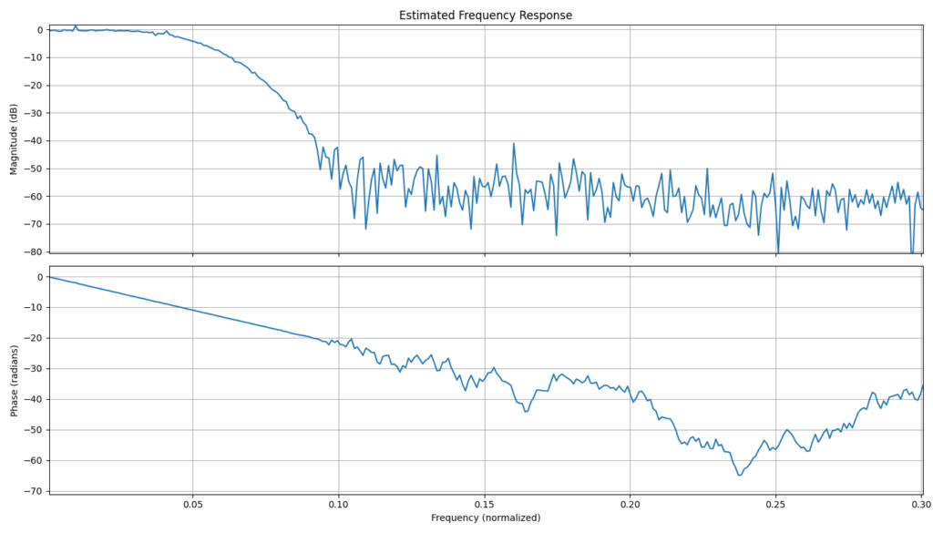
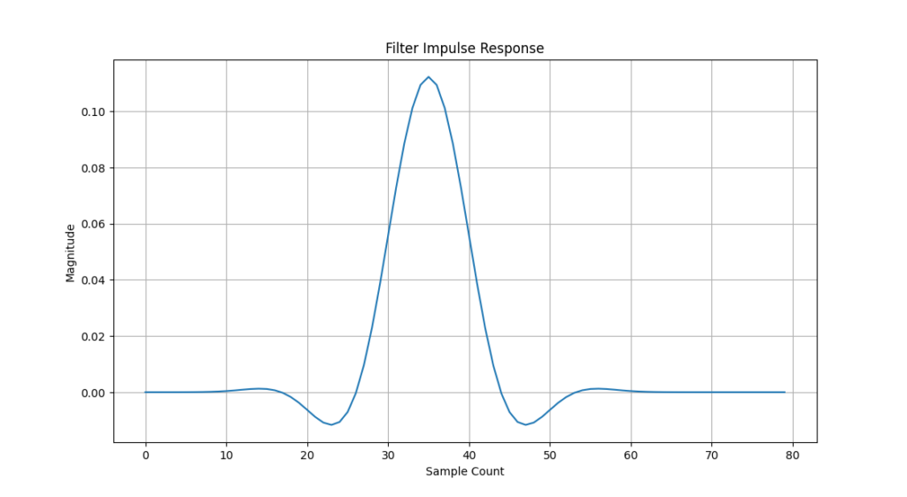
Now the real-time C++ module can be called from Python. The following filter impulse and frequency response estimations and plots provide one example.
import matplotlib.pyplot as plt
import numpy as np

def ImpulseResponse(filterSharpen, num_samples=80):
    output_data = np.zeros(num_samples)
    datum_out   = np.zeros(1)
    datum_in    = np.zeros(1)
    for i in range(num_samples):
        if(i==0):
            datum_in[0] = 1.0
        else:
            datum_in[0] = 0.0
        filterSharpen(datum_out, datum_in)
        output_data[i] = datum_out[0]

    plt.figure(figsize=(14, 6))

    # Magnitude response
    plt.subplot(1, 1, 1)
    plt.plot(output_data)
    plt.title('Filter Impulse Response')
    plt.xlabel('Sample Count')
    plt.ylabel('Magnitude')
    plt.grid()


def FreqResponse(filterSharpen, num_iterations=1000, num_samples=1024):

    # Iteratively send random data through the filter.
    data_length = num_samples
    input_data  = np.zeros(num_samples)
    output_data = np.zeros(num_samples)
    datum_out   = np.zeros(1)
    datum_in    = np.zeros(1)
    H_estimate  = np.zeros(data_length//2)
    for j in range(num_iterations):
        for i in range(num_samples):
            datum_in[0] = np.random.randn()
            filterSharpen(datum_out, datum_in)
            input_data[i] = datum_in[0]
            output_data[i] = datum_out[0]

        if(i==0):
            continue

        # Estimate frequency response using Fourier Transform
        freqs = np.fft.fftfreq(data_length, d=1.0)[:data_length // 2]
        input_fft = np.fft.fft(input_data)[:data_length // 2]
        output_fft = np.fft.fft(output_data)[:data_length // 2]

        H_estimate = H_estimate + output_fft / input_fft

    H_estimate /= (num_iterations - 1)

    # Plot the magnitude and phase response
    fig, (ax1, ax2) = plt.subplots(2, 1, figsize=(14, 8), sharex=True)

    # Magnitude response
    ax1.plot(freqs, 20 * np.log10(np.abs(H_estimate)))
    ax1.set_title('Estimated Frequency Response')
    ax1.set_ylabel('Magnitude (dB)')
    ax1.grid()

    # Phase response (unwrapped)
    ax2.plot(freqs, np.unwrap(np.angle(H_estimate)))
    ax2.set_xlabel('Frequency (normalized)')
    ax2.set_ylabel('Phase (radians)')
    ax2.grid()

if __name__ == '__main__':

    import sigSmart.bin.dsp as dsp

    cfg             = dsp.FilterSharpenPoly10Config()
    cfg.N           = 8  # Larger creates a lower bandwidth.
    filterSharpen   = dsp.FilterSharpenPoly10(cfg, 1)

    ImpulseResponse(filterSharpen)
    FreqResponse(filterSharpen)
    plt.tight_layout()
    plt.show()
Running the above Python code generates the following plots from input/output data processed by the external C++ real-time filter.


Using vcpkg
vcpkg is a general option to simplify installation and management of C++ libraries on Windows, including configuring paths for CMake. In CMakeLists.txt, set CMAKE_TOOLCHAIN_FILE to the path to vcpkg.cmake as follows:
set(CMAKE_TOOLCHAIN_FILE "C:/path/to/vcpkg/scripts/buildsystems/vcpkg.cmake" CACHE STRING "Vcpkg toolchain file")Then on the command line, install pybind11 as follows:
./vcpkg install pybind11which should allow the following to work without any additional configuration:
find_package(pybind11 CONFIG REQUIRED)